9615-07

CIS 9615. Analysis of Algorithms

Greedy Algorithms

1. The idea

Greedy algorithm: optimization by making the locally optimal choice, without looking further.

Examples:

Matrix-Chain Multiplication: in each step, eliminate the largest row/column number. Complexity: O(n lg n).
Optimal Binary Search Tree: in each step, choose a root by considering both probability and balance. Complexity: O(n²).
The Assignment 3 Problem: in each step, choose the smaller cost between moving right and moving down. Complexity: ???

Compared to dynamic programming: faster, though may miss the optimal solution.

Under certain condition, locally optimal decisions do lead to globally optimal decisions.

A problem exhibits "optimal substructure" if an optimal solution to the problem contains optimal solutions to the sub-problems.

2. Example: Activity selection

Problem: for a given set of activities a₁ ... a_n, each a_i using a resource exclusively in interval [s_i, f_i), find a schedule that maximize the number of compatible activities.

Dynamic programming solution: consider S_ij, the set of all activities compatible with a_i and a_j where f_i < s_j, then finally decide the size of the maximum compatible subset of S_0,n+1. For each S_ij, the size of the maximum compatible subset can be obtained by going through all a_k in the set, so to recursively reduce the problem to S_ik and S_kj.

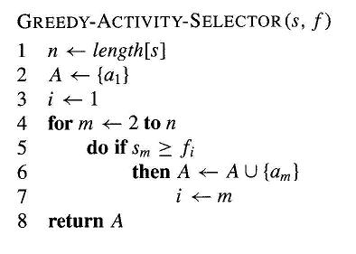
Greedy solution: recursively find the activity that is compatible with the current schedule while having the earliest finish time, and add it into the schedule.

The solution can be proved to be optimal: the earliest-finished activity must be in the optimal solution.

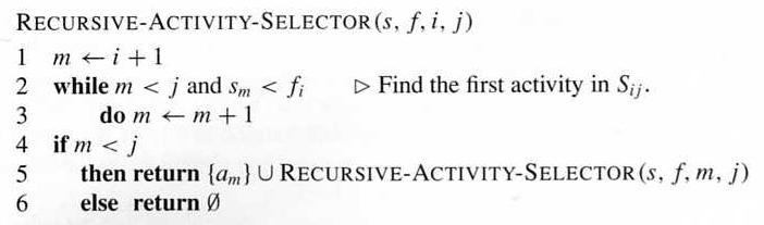
A recursive algorithm initially called as Recursively-Activity-Selector(s, f, 0, n+1), with the activities sorted by finish time.
07-01 (19K)

A more efficient iterative algorithm:
07-02 (14K)
What are the growth orders of these algorithms?

3. Example: Huffman coding

To use variable-length code for data units, with higher-frequent ones with shorter codes.

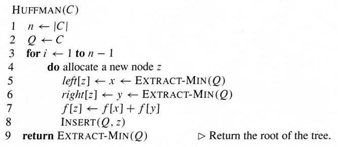
Assuming binary prefix coding, a solution can be represented by a binary tree, with each leaf corresponds to an unit, and its path from root represent the code for the unit. An optimal code is a binary tree with the minimum expected path length.

In the following algorithm, C contains a set of units, and f contains the frequency values of the units. Q is a priority queue, implemented by a heap.

07-03 (23K)

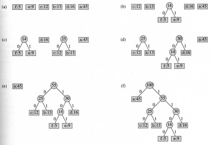
Example:
07-04 (45K)

Demo applet

The running time of the algorithm is O(n lg n): n elements in a min-heap.

Compared to optimal binary search tree: similarity and difference.

4. Related topics

Hill Climbing: when an optimization problem can be represented as searching for the maximum value of a function in a space, "hill climbing" is a greedy algorithm which moves to the local maximum value in each step.

Best-First Search: if the next step is selected at the neighborhood of all explored points, "hill climbing" become "best-first search".