Linear Programming
The Ford-Fulkerson Method finds the maximum flow of a given flow network:
Ford-Fulkerson-Method(G, s, t)
1 initialize flow f to 0
2 while there exists an augmenting path p
3     do augment flow f along p
4 return f
Intuitively, an augmenting path is a path from s to t that still has residual (remaining) capacity, and the additional flow is decided by the edge in the path that has the smallest difference between the flow capacity and the current flow.
Tricky point: a later path can partially "cancel" a previous flow.
The amount of additional flow we can push from u to v before exceeding the capacity c(u, v) is the residual capacity of (u, v), given by
cf(u, v) = c(u, v) - f(u, v)The residual network of G is the graph formed by all the edges with positive residual capacity between every pair of vertices.
Example: Figure 26.5.
When the capacities are integers, the runtime of Ford-Fulkerson is bounded by O(Ef), where E is the number of edges in the graph and f is the maximum flow in the graph. This is because each augmenting path can be found in O(E) time and increases the flow by an integer amount which is at least 1.
When an algorithm follows this method and uses BFS to scan the paths, it becomes Edmonds-Karp algorithm, which runs in O(V E2) time.
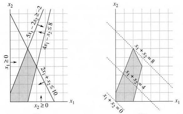
Example: maximize x1 + x2, subject to the following constraints:
  4x1 - x2 ≤ 8
  2x1 + x2 ≤ 10
  5x1 - 2x2 ≥ -2
  x1 ≥ 0
  x2 ≥ 0
Feasible solution: values of x1, x2 that satisfy the constraints — some LP problems have no solution or no optimal solution. Feasible region and objective function of the above problem:
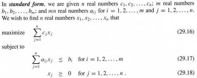
  maximize    cTx  (cT is the transpose of c)
  subject to  Ax ≤ b, x ≥ 0
Consequently, a LP problem in standard form is fully specified by (A, b, c). Any linear program can be converted into the standard form by coefficient negation (minimizing becomes maximizing, and "≤" exchanges with "≥"), variable substitution (every variable can be replaced by the difference of two non-negative variables), and equality-to-inequality-pair replacement (see textbook).
A slack variable defined as s = b - Ax can turn the inequality into an equation, plus the equality s ≥ 0. As a result, the linear program changes from standard form to slack form:
  z = v + cTx
  s = b - Ax
  x ≥ 0
  s ≥ 0
where z is the variable to be maximized, and v is an optional constant. We can also append s into x, while using two index sets to distinguish them: B for s ("basic variables") and N for the original x ("nonbasic variables"). Consequently, a LP problem in slack form is fully specified by (N, B, A, b, c, v).
The simplex algorithm is described in Section 29.3, and in the following it will be explained using a concrete example.
The following LP problem is in standard form:
  maximize   3x1 + x2 + 2x3
  subject to x1 + x2 + 3x3 ≤ 30
             2x1 + 2x2 + 5x3 ≤ 24
             4x1 + x2 + 2x3 ≤ 36
             x1, x2, x3 ≥ 0
convert the problem into slack form:
z = 3x1 + x2 + 2x3
x4 = 30 - x1 - x2 - 3x3
x5 = 24 - 2x1 - 2x2 - 5x3
x6 = 36 - 4x1 - x2 - 2x3
A solution (x1, ..., x6) is feasible if and only if all of the 6 values are nonnegative. The basic solution (0, 0, 0, 30, 24, 36) can be obtained by setting all nonbasic variables to be 0. This solution is feasible, and the value of the objective function for this solution is 0.
In each iteration, the simplex algorithm does a "pivoting", i.e., reformulating the problem to get a better basic solution by selecting a nonbasic variable whose coefficient in the objective function is positive, and turning it into a basic variable. This is the "entering" variable, and the "leaving" (basic) variable is the first one to become negative when the entering variable increases.
When x1 is selected as the entering variable, the leaving variable is x6. The last equation above can be reformulated into
x1 = 9 - x2/4 - x3/2 - x6/4Using it to substitute the other x1 on the right hand side:
z = 27 + x2/4 + x3/2 - 3x6/4
x1 = 9 - x2/4 - x3/2 - x6/4
x4 = 21 - 3x2/4 - 5x3/2 + x6/4
x5 = 6 - 3x2/2 - 4x3 + x6/2
Now the basic solution is (9, 0, 0, 21, 6, 0), and the objective function value is 27.
Do a pivot again to let x3 enter and x5 leave:
z = 111/4 + x2/16 - x5/8 - 11x6/16
x1 = 33/4 - x2/16 + x5/8 - 5x6/16
x3 = 3/2 - 3x2/8 - x5/4 + x6/8
x4 = 69/4 + 13x2/16 + 5x5/8 - x6/16
Now the basic solution is (33/4, 0, 3/2, 69/4, 0, 0), and the objective function value is 111/4.
Do a pivot again to let x2 enter and x3 leave:
z = 28 - x3/6 - x5/6 - 2x6/3
x1 = 8 + x3/6 + x5/6 - x6/3
x2 = 4 - 8x3/3 - 2x5/3 + x6/3
x4 = 18 - x3/2 + x5/2
Now all coefficients in the objective function are negative, so the optimal value is z = 28, which corresponds to solution (8, 4, 0, 18, 0, 0), or x = (8, 4, 0)T in the original form of the problem.
If in a LP problem the feasible solutions corresponds to a distortion of an n-dimensional cube, the worst-case complexity of the simplex algorithm may reach Θ(2n). Nevertheless, it is usually remarkably efficient in practice.