Graph: Optimization
It's relation with the "tree" introduced before, and the related notions.
If G is also weighted, then T is a minimum spanning tree if it has the minimum value of ∑w(u, v) [for (u, v) ∈ T]. It is not necessarily unique.
Finding MST: tree building or cycle breaking.
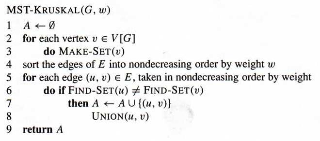
Kruskal's algorithm each time adds an edge that have the least w, and connect two previously unconnected subgraphs. The algorithm uses disjoint-set forest to represent subtrees, and Find-Set(u) identifies the set in which u belongs, which can be done in O(lg E) time (see Section 21.3).
Kruskal's algorithm is a greedy algorithm, and since it processes each edge in order, it takes O(E lg E) time, which can also be written as O(E lg V), given |E| ≤ |V|2.
Prim's algorithm grows a MST by adding vertices one by one into the tree, starting from a root r.
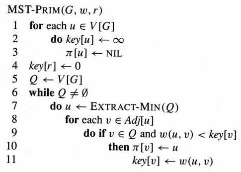
For each vertex v, key[v] is the minimum weight of any edge connecting v to a vertex in the tree. In line 7, Extract-Min(Q) takes the vertex with the lowest key value out of Q.
Prim's algorithm also takes O(E lg V) time. See the textbook for details.
A section of a shortest path is also a shortest path. For graph G = (V, E), the shortest path contains less than |V| edges. If a graph contains a negatively-weighted cycle, then there is no shortest path on that cycle.
If all edges are equally-weighted, the breadth-first search algorithm finds shortest paths from a source vertex to all other vertices. However, it does not work if the edges have different weights.
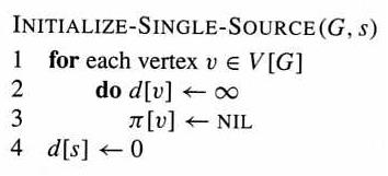
The following algorithm initializes the distance array d and the predecessor array π.
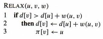
Many shortest-path algorithm use the "relaxation" technique, which tries to improve the shortest distance to vertex v by taking vertex u into consideration, with (u, v) as the last step. The matrix w stores the weights of the edges.
Bellman-Ford algorithm processes the graph |V|–1 passes, and in each pass, tries the edges one-by-one to relax the distance. After that, if there is still possible relaxation, the graph contains negatively-weighted cycle.
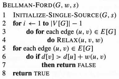
The running time is O(V E), though it can be stopped earlier of a whole loop does not do any update.
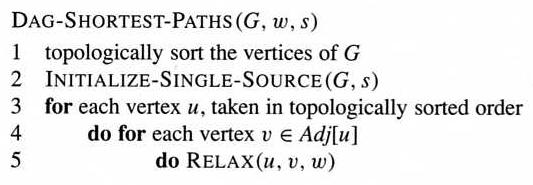
If the graph is a DAG, there are faster solutions. The following algorithm topologically sort the vertices first, then determine the shortest paths for each vertex in that order. It runs in Θ(V + E) time, which comes from topological sorting (and DFS).
Dijkstra's algorithm works for directed graphs without negative weight. It repeatedly selects the vertex with the shorted path, then use it to relax the paths to other vertices.
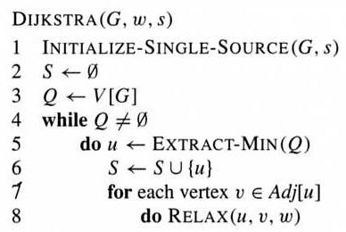
It is similar to MST-Prim, except here the distance is to the starting vertex, not to the MST.
Comparison among the above three algorithms.
Floyd-Warshall algorithm uses dynamic programming, and in each step adds one possible intermediate vertex into the shortest paths.
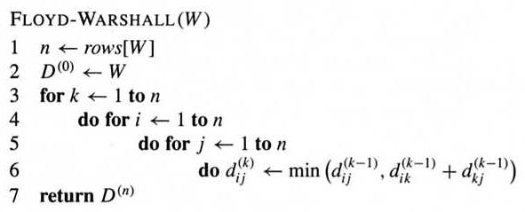
The running time of the above algorithm is Θ(n3).
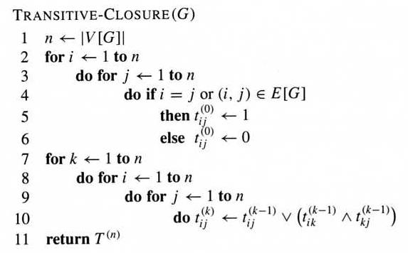
A similar algorithm calculates the transitive closure of a graph, where T(n)ij = 1 if and only if there is a path from i to j.