CIS 307: Performance Evaluation
Introduction
Engineers do it. Cooks do it. But seldom programmers do it. What is it?
It is good Performance Evaluation of either an existing system or of
its design.
If an engineer estimates the need for steel in a building as a hundred
tons when two hundred are called for, he will be laughed at (or worse).
If a cook doubles the correct amount of spices in a dish, he is likely
to lose clients. But if a programmer makes estimates that are orders of
magnitude off, he feels that nothing extraordinary has happened and
many other programmers are likely to feel the same.
Yet it is not too difficult to come up with performance estimates
of times and sizes that are
fairly accurate (from 50% off to only a few % off). Thoughout this course I
do simple computations, often not more complicated than additions and
multiplications, to estimate some performance factor of a system. In your
first homework you have used a complex method of performance evaluation:
discrete-event simulation. Other methods of performance evaluation are
analytical, some involving sophisticated math like Markov models, other
are simple, as we shall now see.
Saturation and BottleNecks
We say that a server is saturated, or that it has reached
saturation when its utilization is 100% (i.e. it is busy
all the time; utilization is the ratio between the time a server is in
use and the total time). For example, if a disk takes 10msec to service a
request,
it will saturate when it receives 100 requests per second.
[More in general, people say that a server is saturated when its service
becomes inacceptable, and that may happen at a 80% utilization. However
for our purposes in this note we will stick to the 100% figure.]
If a system
has many servers, we can then talk of its bottleneck, that is, of
the server that will saturate first as the load on the system increases.
Once the bottleneck saturates, also the system will saturate, i.e. it will
not be able to handle any greater load. The bottleneck of the system determines
the throughput (number of jobs completed per unit of time) of the
system. [This discussion
assumes that we have jobs that have all the same characteristics].
Example 1: In the following system

we can execute jobs. Each job first does READ, then moves to PROCESS, then
moves to PRINT. These three phases are independent of each other in the
sense that a job can be reading while another is processing and another is
printing. Assume that a job takes 1 second to read, 4 seconds to process, and
2 seconds to print. Question: What is the (best possible) response time
[response time is the time interval from the moment that a job arrives to
the moment it exits]? Answer: 7 seconds. Question: What is the
bottleneck in this system? Answer: the PROCESS phase.
Question: How many jobs can be completed per minute (at most)?
Answer: 15.
This was an example of servers placed in sequence. In a serial or sequential
arrangement the throughput of the sequence is equal to the smallest
throughput of a server in the series.
Example 2: In the following system

jobs require a total of 100msec of compute time and require 20
operations on the disk whose service time is 10msec.
Question: What is the minimum response time? Answer: 300msec.
Question: What is the
bottleneck in this system? Answer: The disk. Question: What is the throughput
of the system (you can assume that a job can be computing while another
is waiting for IO)? Answer: 5 jobs per second.
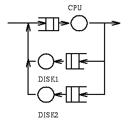
Example 3: In the following system

jobs require a total of 100msec of compute time, require 20 IO operations
on Disk 1 (whose service time is 10msec), and 50 IO operations on Disk 2
(whose service time is 5msec).
Question: What is the minimum response time? Answer: 550msec.
Questions: What is the bottleneck? Answer:
Disk 2. Question: What is the throughput? Answer: 4 jobs per second.
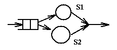
When servers are placed in parallel and a job can use either server, then
the maximum throughput of the system becomes equal to the sum of the maximum throughputs
of the individual servers. For example in the following system

assume that S1 has a throughput of 3 jobs per second and S2 a throughput of
2 jobs per second. Then the system has a total maximum thoughput of 5 jobs
per second. The minimal response time will be 1/3 of a second. The
average response time is harder to compute (we assume no queueing):
in one second 3 jobs will have a response time of 1/3sec and 2 jobs
a response time of 1/2sec; thus the average response time is
(3/5*1/3+2/5*1/2),
i.e. 2/5sec. In the case of servers in parallel it is not evident what
represents the bottleneck of the system: though in our example S2 will
saturated before S1, the system as a whole does not saturate at that time.
In the case of parallel servers the question of saturation requires
additional assumptions about the use and cost of the servers.
Little's Law
Little's Law applies to the single server queueing system (a server and
its queue). It is the equation:
N = a * T
where:
- N is the number of jobs in the queueing system (queue plus server)
- a is the arrival rate (the number of jobs that arrive to the system per
unit of time), and
- T is the Response or TurnAround Time for a job (total time from arrival to
departure from the system).
For example, if at the supermarket I notice that a teller has always 4
customer and that customers arrive every 2 minutes, then I know that
customers, on average will be in line for 8 minutes.
Little's Law has an intuitive foundation and it can be proven under
general assumptions as to the arrival rate of jobs, as to the service rate, and
as to the scheduling discipline. One can use it reliably.
Notice that if we are given the average time spent by
a job on the server, i.e. the service time Ts,
and the average inter-arrival time Ta,
then we
can compute the utilization of the server: Ts/Ta.
If we let inter-arrival rate = a = 1/Ta then we have the relation
utilization = a*Ts, which is called the Utilization Law
.
Response Time in the M/M/1 Queueing System
One can do a mathematical analysis of a Single Server
Queueing System where arrival times are Poisson distributed and
service times are exponential. These systems are called
M|M|1 systems. We say that the arrivals are Poisson
distributed if the probability of K arrivals in time t
is
Pr[X=k, t] = (a*t)k * e-a*t / k!
It corresponds to the situation where all arrivals are independent of each
other and each arrival may occur with equal probability in any interval
t..t+dt. In this formula 'a' represents the average arrival rate.
We say that the service times are exponential when the probability
that the service time is less than x is given by:
Pr[X<=x] = 1 - e-a*x
An interesting relation between Poisson Distribution and Exponential
Distribution is that the the latter can be obtained from the former.
Consider the probability of at least one arrival in the interval t.
This probability is
1 - Pr[X=0, t] = 1 - e -a*t
It is important to realize that in a single server system the arrival rate
must be smaller than the service rate (i.e. a must be smaller than b)
otherwise jobs will arrive faster into the system than the server can take care of them.
For the M|M|1 system we can determine the average response time.
It is given by the formula
	T = ServiceTime/(1-Utilization) =
          = ServiceTime/(1 - ServiceTime/InterArrivalTime) =
          = ServiceTime * InterArrivalTime / (InterArrivalTime - ServiceTime) =
          = 1 / (ServiceRate - ArrivalRate)
In other words, as the utilization reaches 1, i.e. as the server saturates,
the response time goes to infinity. It practice things are not usually
this bad.
This result should give you a feeling
of how dangerous it is to operate in a system where some component is
saturated. In essence the saturated component (the bottleneck) forces
the serialization of each job, that is, each job through the bottleneck
has to wait for the completion of the job that preceded it. If we add
one more arrival in the unit of time, then the response time of each job
is increased by the service time for the bottleneck of this additional job.
The increment would have been less if the bottleneck were not saturated.
In the above formula we can express the Utilization as the ratio
    Arrival Rate                                   Service Time
    ------------ = Arrival Rate * Service Time = ----------------
    Service Rate                                 Interarrival Time
The utilization represents the average number of jobs on the server (at times
the server is idle, the number of jobs is 0, at times the server is busy,
the number of jobs is 1; the average is the Utilization).
The average number of jobs in the queue is easily determined:
JobsInQueue = JobsInSystem - JobsOnServer =
            = N - Utilization = a*T - Utilization =
	    = a * (Ts/(1 - Utilization)) - Utilization
As to the time spent by a job in the queue we have:
JobTimeInQueue = JobTimeInSystem - JobTimeOnServer =
	       = Ts/(1 - Utilization) - Ts =
	       = Utilization * Ts/(1 - Utilization) =
	       = Utilization * JobTimeInSystem
This discussion allows us to arrive at a couple of insights:
- What happens to a system if we double arrival rates and service rates?
May be one would think that Response Time and Average Queue size will not
change. In reality as you can see from the formula, the response time is
halved. As for the queue size, using Little's Law, we see that
it remains unchanged (the arrival rate has doubled but the response time
has halved).
- What happens if we double the power of the server? The response time
is better than halved. Suppose for example that
the current utilization is 80%. Then the old
response time was
        Ts
    -------- = 5*Ts
     1 - 0.8
and the new response time will be
    0.5*Ts
    -------  ~ 0.8*Ts
    1 - 0.4
with an improvement that is by more than a factor of 5.
Here is a numerical example. Suppose we are given a disk where the
service time is 10ms and where requests arrive every 12 ms.
Question: what is the average queue size?
Utilization = 10/12 = 0.83.
T = Ts/(1 - Utilization) = 10/(1 - 0.83) = 10/0.17 = 60
Nqueue = N - Utilization = a*T - Utilization = 1/12*60 - 0.83 = 4.17
Response Time in Round Robin Scheduling
We have seen that RR scheduling involves a quantum q. A running
process, after q seconds, is pre-empted and
placed at the end of the ready queue.
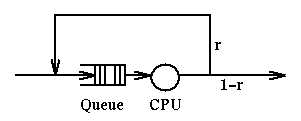
Let's assume that a process, upon completion of a quantum, has probability
r of having to run again (thus, probability 1-r of being terminated).
r is often called a Routing Probability ("route" as in which direction
to go).
How long, in total, will this program run? We can represent this system
with a picture:

If we define g(i) as the probability that a job will go i times through the
server, we have:
g(i) = (1-r)*ri-1
and the expected service time for the process, E(S), will be weighted average
of the number of quanta used at the server, say i, times the probability of
that many iterations, g(i). That is, E(S) is the sum for i from 1 to infinity
of i*q*g(i) which is:
E(S) = q/(1-r)
This assumes that there is no waiting time in the queue, i.e. that there
is no competition for the services of the server. A more difficult question,
left unanswered, is how long will it
take in this system for a job to terminate in the case that m jobs
arrive simultaneously?
Interestingly, the study of transmission in a lossy channel, where the
the transmission takes time q and the probability of loss is r (hence the
message needs to be retransmitted), results in a total
transmission time that is again q/(1-r).
The Five-Minutes Rule
The Five-Minutes Rule is used to evaluate when to cache in memory a
frequently accessed object stored on disk. The idea is to compare the
cost of memory required to store the information, and the cost of
accessing the information from disk.
Suppose I am give a disk that costs $100 and where I can perform
100 accesses per second. That means that the ability to access disk
once per second costs me $1. Assume that a page on disk is accessed
every n seconds, thus the cost of accessing that page is 1/n dollars.
Assume that a megabyte consists of, say, 256 pages
(i.e. 4KB pages), and that 1 MB of memory costs $1. Thus to keep a
page in memory costs 1/256 Dollars. When the cost of keeping the
page in memory is smaller than the cost of accessing the page on
disk, we should cache the page. This happens when, in our example
1/256 < 1/n
that is
n < 256
that is if we access the page at least every 256 seconds, or about 5
minutes.
This same type of reasoning can be applied in a variety of
situations, to trade communication costs and replication costs.
Computational Speedup
Suppose we run a program using a single processor and it takes time T(1). We then run the program using n processors
(we assume the program is written to take advantage of the available number of processors) and it takes time T(n).
What is the relationship between T(1), T(n) and n? For example, if the program takes 100sec on one processor, how
long should it take on four processors? May be 25sec? in fact T(n) at best should be T(1)/n. [Cases where T(n) is less
than T(1)/n, i.e. in our example less than 25 seconds, are called cases of superlinearity. Such cases can be explained
and analyzed separately in terms of OS or computational characteristics. For example, a large program split into 4 parts
running independently may have in the parts a smaller, more easily accomodated working set.]
We call Computational Speedup s the ratio:
s = T(1)/T(n)
and Efficiency e the ratio:
e = s/n
Amdhal has suggested that any computation can be analyzed in terms of a portion that must be executed sequentially,
Ts, and a portion that can be executed in parallel, Tp. Then
T(n) = Ts + Tp/n
This is known as Amdhal's Law. It says that we can improve only the parallel part of a computation. Going back to
our example, if the computation requires 40 seconds of sequential computation and 60 of parallel computation, then the
best that T(n) will ever be is 40sec, even for n growing to infinity. In practice there are many problems where the
sequential components are minimal and thus these problems can be effectively parallelized. In general though speedup
due to parallelism tends to be not too great. Some people suggest that the speedup grows with the square root of n, i.e,
if we quadruple the number of processors, we only double the performance. [Notice that in this case efficiency will
change as 1 over the square root of n, i.e. the more the processors, the less efficiently they will be used.] The maximum
speedup assuming Amdhal's Law is for n going to infinity. That is
s = (Ts + Tp)/Ts = 1 + Tp/Ts
For example, if we are given a program that takes 40 minutes to complete on
a single processor and we are told that for this program Ts is 10m and Tp is 30m then,
if we have 5 processors the speedup will be 40/16 = 2.5 and the efficiency 0.5.
The maximum speedup possible (when we use an infinite number of processors)
is 4. Of course in that case the efficiency becomes 0.
Note that in the speedup we see an application of the Law of
Diminishing Returns. In the case above if we use 2 processors, the time
required becomes 25m, with a percentual gain due to the additional processor
of 15/40, i.e. 37%. If we go from 2 to 3 processors, now the time becomes 20
minutes, with an improvement from 25 of 20%, and if we go to 4 processors
we go to 17.5 minutes, with an improvement of 12.5%, i.e. the
percentual of improvement for each additional machine keeps getting
smaller and smaller.
It has been seen experimentally that Amhdal's Law works well for certain kinds
of computations only, namely in cases of control parallelism, i.e.
where the algorithm can be seen as divided in a number of different
activities that can be done in parallel. It does not work as well in the
case of data parallelism, i.e. in cases where the same operations
can be applied in parallel to different data. In the latter case Amhdal's
predictions are very pessimistic. For this case has been proposed the
Gustafson-Barsis Law. It is based on the observations
      T(n) = Ts + Tp
      T(1) = Ts + Tp/n
Operational Analysis
We can analyze the behavior of Queueing Networks (i.e. networks of queues
and their servers) using fairly simple means. We will examine this topic by
example.
Example 1
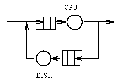
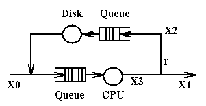
We have the
following queueing network which represents a computer system with a CPU
and a disk. When a job enters the system it goes to the CPU, whence it goes
either to disk (an IO request) or terminates. Upon completion of the IO
operation the job goes back to the CPU and things are repeated.

X0 represents the number of jobs entering the system per unit of time;
X1 represents the number of jobs exiting the system per unit of time;
X2 represents the number of jobs going to disk per unit of time;
X3 represents the number of jobs going to the CPU per unit of time.
At steady state (i.e. when the system displays the same behavior for long
periods of time) we can assume that X0=X1. By observation we determine that
in the system are present in total N jobs at a time. The service times
at the CPU and at the disk are respectively Sc and Sd.
Here are the relations that will hold in this system:
- X0+X2 = X3, because of continuity at the fork going to disk and to the exit
- X2 = r*X3, because of definition of r, X2 and X3
- N = X0*R, where R is the Response Time for this system, because
of Little's Law.
We can use these relations any way we want to compute, given the values
of some variables, the values of the remaining variables.
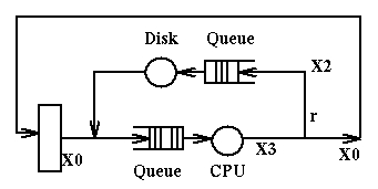
Example 2
Example 2 is very similar to example 1. But now the users of the systems are
all sitting at terminals. Each user request constitutes a job.

We assume:
- Each user request generates v = 20 disk requests
- Disk utilization u is 50%
- Service Time at the disk is Sd = 25ms
- There are M terminals, M = 25
- When a user receives a response, thinks for Z = 18 seconds before
submitting the next request
Question: What is the response time R? We use the equations:
- M = (R+Z)*X0, by Little's Law
- X2 = v*X0, by definition of v, X0, X2
- u = X2 / (1/Sd), by definition of u, X1, Sd
Then we get easily our response time:
- X2 = u/Sd = 0.5/0.025 = 20
- X0 = X2/v = 20/20 = 1
- R = M/X0 - Z = 25/1 - 18 = 7
Notice that it is easy to determine the maximum possible value of X2, the
saturation value, that is reached when the disk is fully utilized.
Since the service time of the disk is 25ms, the maximum value of X2 is 40
[since in a second we can have at most 40 disk operations].
As you have seen from these examples, simple performance evaluation is
very feasible, using intuition and simple math.
ingargio@joda.cis.temple.edu
