Graph: Structure Exploration
Formally, a graph G = (V, E), where V is a set of vertices, and E is a set of edges (from a vertex to a vertex), so |E| ≤ |V|2. The "size" of G is usually represented by both |V| and |E|, with respect to which the computational complexity of graph algorithms is represented.
Tree structures and linear structures are special cases of graph structures.
A graph may either be directed or undirected, depending on whether the relation is symmetric or not.
A graph is connected if there is a path from every vertex to every other vertex. Specially, a directed graph is strongly connected if there is a (directed) path from every vertex to every other vertex; otherwise, it is weakly connected if the graph is connected after all directed edges are turned into undirected edges.
A graph is weighted if every edge has a number associated.
Beyond graph: hypergraph, labeled graph, multigraph.
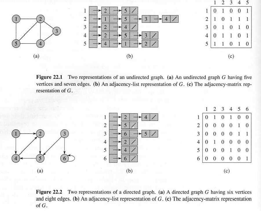
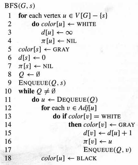
The two common ways to represent a graph is by an adjacency matrix and by an adjacency list. Both can be expended to represent weighted graph.
Space and time costs: the former is better for dense graphs, while the latter is better for sparse graphs. In adjacency matrix, predecessor and successor are symmetric, while in adjacency list they are not.
For graphs with additional properties, special-purpose representation may be more efficient.
Breadth-First Search (BFS): starting from a source vertex, visits its neighbors layer-by-layer with increasing distance. The algorithm represents a graph using adjacency list, with a queue used to hold the nodes under processing. A "color" is attached to every node to indicate its status: to be processed (white), being processed (gray), have been processed (black). For each node, its predecessor and distance are recorded (on the path from the source node).
Example:
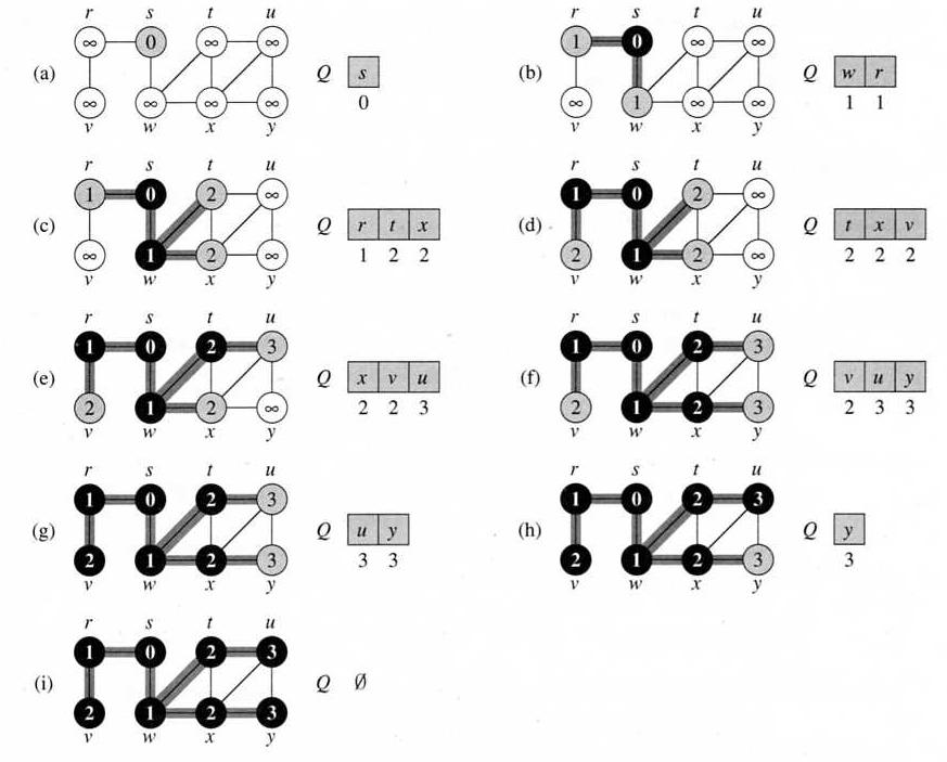
Under the assumption that all nodes can be reached from the source node, the running time of BFS is Θ(V + E), since it spends constant amortized cost on each node (enqueue/dequeue) and each link (follow the adjacency list).
As a by-product, this algorithm also generates a (breadth-first) search tree with s as root, and find the shortest path between s and every reachable vertex in G.
If in search, the algorithm tries to go as deep as possible in each step, then it is a Depth-First Search (DFS) algorithm.
The above BFS algorithm can be changed into a DFS algorithm by simply changing the queue into a stack, each time only processing one successor of the node at the top of the stack, and backtracking to a previous node if the top one has been fully processed.
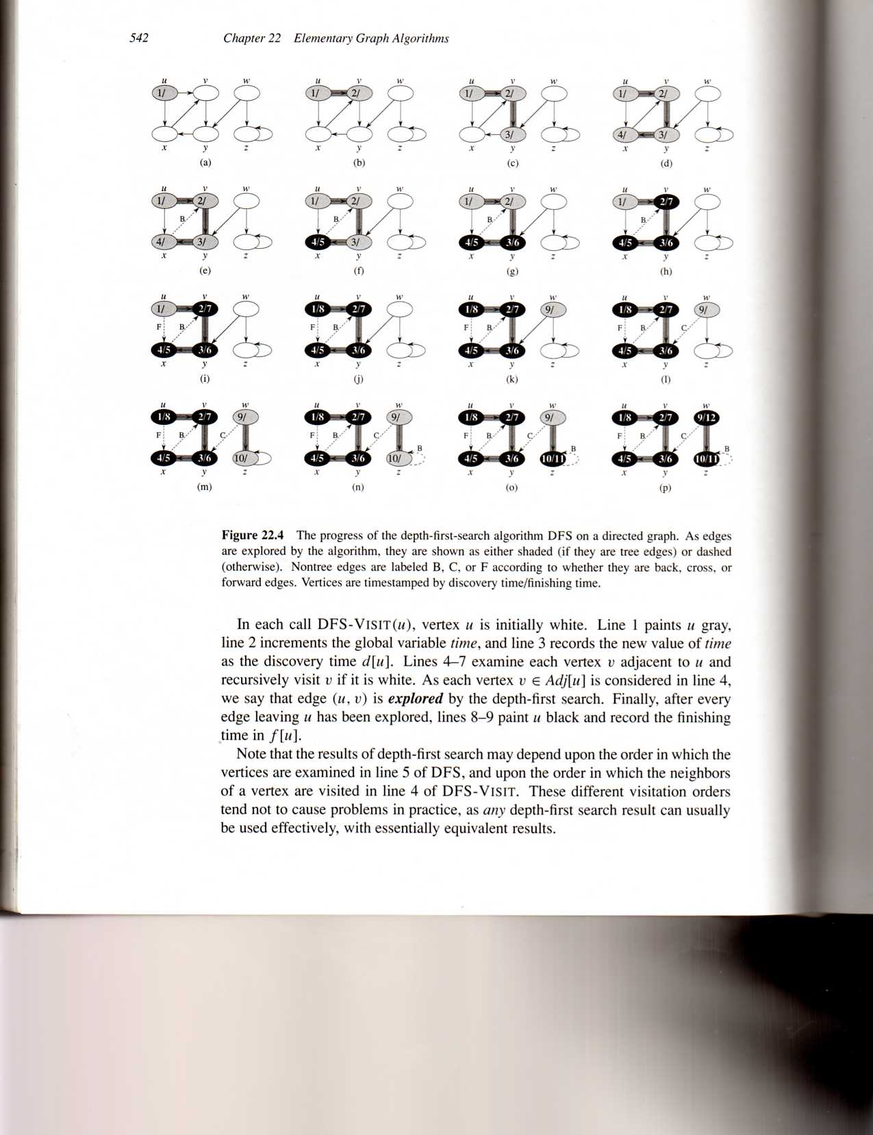
The following is a recursive DFS, which uses two time-stamps, d and f, to record the time of color changing for each vertex. This information will be used in the other algorithms to be introduced later.
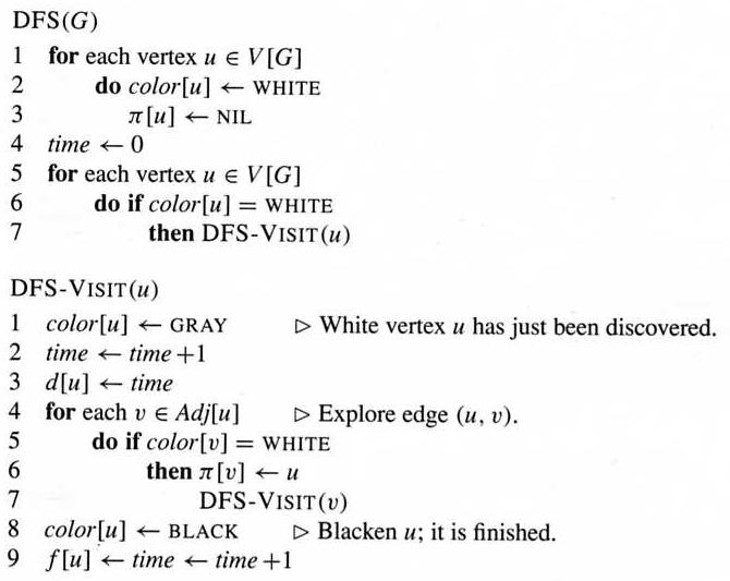
Example: Figure 22.4
The running time of DFS is also Θ(V + E), though this algorithm does not assume the connectivity of the graph, so may produce a forest consisting of multiple depth-first trees.
The ascendant-descendant relation between nodes in the forest corresponds to the inclusion of their time intervals. Classification of edges by color or clock.
The following algorithm uses DFS to do topological sorting in dags:
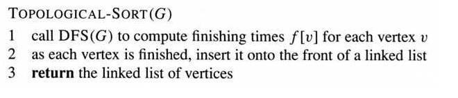
Please note that it is the finishing order, not starting order, of the nodes that matters. Example.
The algorithm takes Θ(V + E) time.
The algorithm can be revised to detect cycle: see Lemma 22.11.
A more natural solution for topological sorting is to repeatedly remove a node that has no predecessor (or successor).
Strongly connected components in a directed graph: example. Component graph (meta-graph).
Basic ideas: repeatedly removing (or marking) "sink" components using DFS-Visit.
The "sink" component of G is the "source" component of the transpose of G, and vice versa.
To identify a vertex in a "source" component: look for the largest f number, which is a vertex without predecessor outside the component.